One way of obtaining resistant statistics is to use
the empirical quantiles (percentiles/fractiles).
The quantile (this term was first used by Kendall, 1940) of
a distribution is the number ![]() such
that a proportion
such
that a proportion ![]() of the values are less
than or equal to
of the values are less
than or equal to ![]() . For example, the 0.25 quantile
. For example, the 0.25 quantile ![]() (also referred to as the 25th percentile or lower quartile)
is the value such that 25% of all the values fall below that value.
(also referred to as the 25th percentile or lower quartile)
is the value such that 25% of all the values fall below that value.
Empirical quantiles can be most easily constructed by
sorting (ranking) the data into ascending order to obtain a sequence of
order statistics
![]() as shown in Figure 2.1b.
The
as shown in Figure 2.1b.
The ![]() 'th quantile
'th quantile ![]() is then obtained by taking the rank
is then obtained by taking the rank ![]() 'th
order statistic
'th
order statistic
![]() (or an average of neigbouring values if
(or an average of neigbouring values if
![]() is not integer):
is not integer):
![$\displaystyle \left\{ \begin{array}{ll}
x_{((n+1)p)} & \mbox{ if $(n+1)p$\ is i...
...\\
0.5*(x_{([(n+1)p])}+x_{([(n+1)p]+1)}) & \mbox{otherwise}
\end{array}\right.$](img33.png) |
(2.5) |
Unlike the arithmetic mean, the median ![]() is not at all influenced by
the exact value of the largest objects and so provides a resistant
measure of the central location.
Likewise, a resistant measure of the scale can be obtained using the
Inter-Quartile Range (IQR) given by the difference between the
upper and lower quartiles
is not at all influenced by
the exact value of the largest objects and so provides a resistant
measure of the central location.
Likewise, a resistant measure of the scale can be obtained using the
Inter-Quartile Range (IQR) given by the difference between the
upper and lower quartiles
![]() .
In the asymptotic limit of large sample size (
.
In the asymptotic limit of large sample size (
![]() ),
for normally (Gaussian) distributed variables (see Chapter 4),
the sample median tends to
the sample mean and the sample IQR tends to 1.34 times the
sample standard deviation.
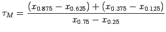
Resistant measures of skewness and kurtosis also exist
such as the dimensionless Yule-Kendall skewness statistic
),
for normally (Gaussian) distributed variables (see Chapter 4),
the sample median tends to
the sample mean and the sample IQR tends to 1.34 times the
sample standard deviation.
Resistant measures of skewness and kurtosis also exist
such as the dimensionless Yule-Kendall skewness statistic
 |
(2.6) |