


Next: Alternative hypotheses
Up: Statistical hypothesis testing
Previous: Getting rid of straw
Contents
Figure:
Schematic showing the sampling density function of a test statistic
assuming a certain null hypothesis. The critical levels are shown
for an (unusually large) level of significance
 for
visually clarity.
for
visually clarity.
|
Statistical testing generally uses a suitable
test statistic  that can be calculated
for the sample. Under the null hypothesis, the test statistic
is assumed to have a sampling distribution that tails
off to zero for large positive and negative values of
that can be calculated
for the sample. Under the null hypothesis, the test statistic
is assumed to have a sampling distribution that tails
off to zero for large positive and negative values of  .
Fig. 6.1 shows the sampling distribution of a typical test
statistic such as the Z-score
.
Fig. 6.1 shows the sampling distribution of a typical test
statistic such as the Z-score
 , which is used to test hypotheses about
the mean. The decision-making procedure in classical statistical inference
proceeds by the following well-defined steps:
, which is used to test hypotheses about
the mean. The decision-making procedure in classical statistical inference
proceeds by the following well-defined steps:
- Set up the most reasonable null hypothesis
- Specify the level of significance
 you are prepared to accept.
This is the probability that the null hypothesis will be rejected even
if it really is true (e.g. the probability of convicting innocent
people) and so is generally small (e.g. 5%).
you are prepared to accept.
This is the probability that the null hypothesis will be rejected even
if it really is true (e.g. the probability of convicting innocent
people) and so is generally small (e.g. 5%).
- Use
 to calculate the sampling distribution
 of your desired test statistic
- Calculate the p-value
 of your observed sample value of the test statistic.
The p-value gives the probability of finding samples of data
even less consistent with the null hypothesis than your
particular sample assuming is true
i.e. the area in the tails of the probability
density beyond the observed value of the test statistic.
So if you observe a particularly large value
for your test statistic, then the p-value will be very small since
it will be rare to find data that gave even larger values for
the test statistic.
of your observed sample value of the test statistic.
The p-value gives the probability of finding samples of data
even less consistent with the null hypothesis than your
particular sample assuming is true
i.e. the area in the tails of the probability
density beyond the observed value of the test statistic.
So if you observe a particularly large value
for your test statistic, then the p-value will be very small since
it will be rare to find data that gave even larger values for
the test statistic.
- Reject the null hypothesis if the p-value is less than the level
of significance
 on the grounds that the data are
inconsistent with the null hypothesis at the level
of significance. Otherwise, do not reject the null hypothesis
since the ``data are not inconsistent'' with it.
on the grounds that the data are
inconsistent with the null hypothesis at the level
of significance. Otherwise, do not reject the null hypothesis
since the ``data are not inconsistent'' with it.
The level of significance defines a rejection region
(critical region) in
the tails of the sampling distribution of the test statistic.
If the observed value of the test statistic lies in the
rejection region, the p-value is less than and
the null hypothesis is rejected.
If the observed value of the test statistic lies closer to the
centre of the distribution, then the p-value is greater than
or equal to and the null hypothesis can not be rejected.
All values of that have p-values greater than or equal to
define the
 confidence interval.
Example: Are meteorologists taller or shorter than other people ?
Let us try and test the hypothesis that Reading meteorologists have
different mean heights to other people in Reading based
on the small sample of data presented in Table 2.1.
Assume that we know that the population of all people in
Reading have heights that are normally distributed with
a population mean of  170cm and a population standard deviation
of
170cm and a population standard deviation
of  30cm. So the null hypothesis is that our sample of meteorologists
have come from this population, and the alternative hypothesis
is that they come from a population with a different mean height.
Mathematically the hypotheses can be stated as:
30cm. So the null hypothesis is that our sample of meteorologists
have come from this population, and the alternative hypothesis
is that they come from a population with a different mean height.
Mathematically the hypotheses can be stated as:
 |
|
|
(6.1) |
 |
|
|
|
where  cm. Let's choose a typical
level of significance equal to 0.05.
Under the null hypothesis, the sampling distribution
of sample means should follow
cm. Let's choose a typical
level of significance equal to 0.05.
Under the null hypothesis, the sampling distribution
of sample means should follow
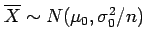 ,
and hence the test statistic
,
and hence the test statistic
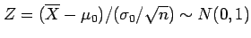 .
Based on our sample of data presented in Table 2.1,
the mean height is
.
Based on our sample of data presented in Table 2.1,
the mean height is
 and so the test statistic
 is equal to 0.48, in other words, the mean of our sample
is only 0.48 standard errors greater than the population mean.
The p-value, i.e. the area in the tails of the density curve
beyond this value, is given by
is equal to 0.48, in other words, the mean of our sample
is only 0.48 standard errors greater than the population mean.
The p-value, i.e. the area in the tails of the density curve
beyond this value, is given by
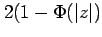 and so for a
of 0.48 the p-value is 0.63, which is to say that there
is a high probability of finding data less consistent with
the null hypothesis than our sample.
The p-value is clearly much larger than the significance level
and so we can not reject the null hypothesis in this case -
at the 0.05 level of significance, our data is not
inconsistent with coming from the population in Reading.
Based on this small sample data, we can not say that
meteorologists have different mean heights to other people
in Reading.
and so for a
of 0.48 the p-value is 0.63, which is to say that there
is a high probability of finding data less consistent with
the null hypothesis than our sample.
The p-value is clearly much larger than the significance level
and so we can not reject the null hypothesis in this case -
at the 0.05 level of significance, our data is not
inconsistent with coming from the population in Reading.
Based on this small sample data, we can not say that
meteorologists have different mean heights to other people
in Reading.
Next: Alternative hypotheses
Up: Statistical hypothesis testing
Previous: Getting rid of straw
Contents
David Stephenson
2005-09-30