It is often the case that a response variable may depend on more than one explanatory variable. For example, human weight could reasonably be expected to depend on both the height and the age of the person. Furthermore, possible explanatory variables often co-vary with one another (e.g. sea surface temperatures and sea-level pressures). Rather than subtract out the effects of the factors separately by performing successive iterative linear regressions for each individual factor, it is better in such cases to perform a single multiple regression defined by an extended linear model. For example, a mutliple regression model having two explanatory factors is given by
| (8.1) |
This model can be fit to the data using least squares
in order to estimate the three ![]() parameters. It
can be viewed geometrically as fitting a
parameters. It
can be viewed geometrically as fitting a
![]() dimensional hyperplane to a cloud of points
in
dimensional hyperplane to a cloud of points
in
![]() space.
space.
The multiple regression equation can be rewritten more concisely in matrix notation as
| (8.2) |
The least squares solution is then given by the set of
normal equations
| (8.3) |
As with many multivariate methods, a good understanding
can be obtained by considering the bivariate case with two
factors (![]() ). To make matters even simpler, consider the
unit scaled case in which
). To make matters even simpler, consider the
unit scaled case in which ![]() and
and ![]() have been
standardized (mean removed and divided by standard deviation)
before performing the regression.
By solving the two normal equations, the best estimates for
the beta parameters can easily be shown to be given by
have been
standardized (mean removed and divided by standard deviation)
before performing the regression.
By solving the two normal equations, the best estimates for
the beta parameters can easily be shown to be given by
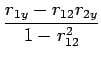 |
(8.4) | ||
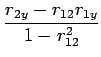 |
(8.5) |
| (8.6) | |||
| (8.7) |
The MINITAB output below shows the results of multiple regression of height on weight and age for the sample of meteorologists at Reading:
The regression equation is
Weight = - 40.4 + 0.517 Age + 0.577 Height

Predictor       Coef    StDev       T       P
Constant      -40.36    49.20   -0.82   0.436
Age           0.5167   0.5552    0.93   0.379
Height        0.5769   0.2671    2.16   0.063

S = 6.655       R-Sq = 41.7%     R-Sq(adj) = 27.1%

Analysis of Variance

Source          DF      SS      MS      F       P
Regression       2      253.66  126.83  2.86    0.115
Residual Error   8      354.34   44.29
Total           10      608.00
It can be seen from the p-values and coefficient of determination
that the inclusion of age does not improve the fit compared to the
previous regression that used only height to explain weight. Based
on this small sample, it appears that at the 10% level
age is not a significant factor in determining body weight
(p-value
![]() ), whereas height is a significant factor
(p-value
), whereas height is a significant factor
(p-value
![]() ).
).