Worm Simulation in square grid with 8 paths and diagonals
Neil Vaughan
Abstract
This research presents a computer simulation model of worms tracing paths as they move through sediment. A new type of 2D square grid with 8 paths including diagonals is used which has not been modelled before. The results include many interesting and intricate patterns traced by the worms. In this grid, there are a very large number of worms, potentially around 10^33. A substantial number of worms have been modelled up to 12 million population size in this research and some images are shown. A large uncountable number of worms remain with an unknown outcome in category R because eithere there are too many worms to model, or the worms continue running for too many millions of steps before becoming a category L or T.
Introduction to the 8 path model
A 2D model with 8 paths has never been used in literature on worm simulation. The diagrams in Fig. 1a-g show how the proposed 2D square grid with diagonals works. At each point in the 2D grid, there are 8 gridlines joining at each vertex. This provides a choice of up to 7 directions per step, diagonal moves are not allowed. The system uses 2 axes of movement: x and y.
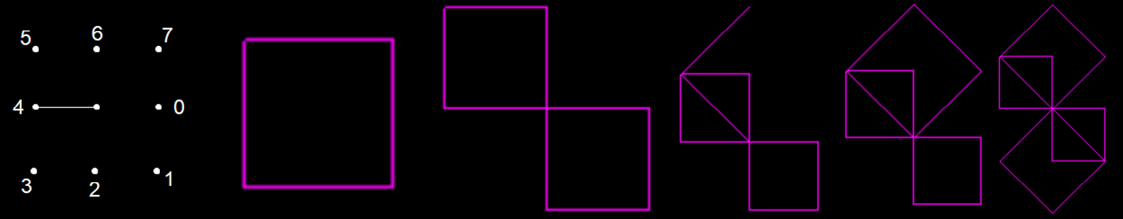
Fig. 1. (a) The 2D square with diagonal grid system to simulate worm path movement. (b-f) Five stages detailing the growth process of a trail produced by a simple example worm (26326) with five rules, which terminates in category N with population 16.
Rules of Worm Simulations
[Beeler, 1973]
- A worm cannot re-trace any path that it has traversed previously.
- Worms detect which paths are available at each step, and based on the path availability, they choose a direction to turn and they store their decision in memory.
- In future, if the exact same distribution of available paths is encountered again, the same turn decision must be made again.
- If the worm gets to a dead-end situation where 0 paths are available, it automatically terminates.
- If only one path is available, that path is taken without setting a new rule.
- The axes of rotation (Fig. 1h) rotate with the worm, so that path 0 always means move straight ahead and path 4 is always unavailable due to already having been traversed.
Results
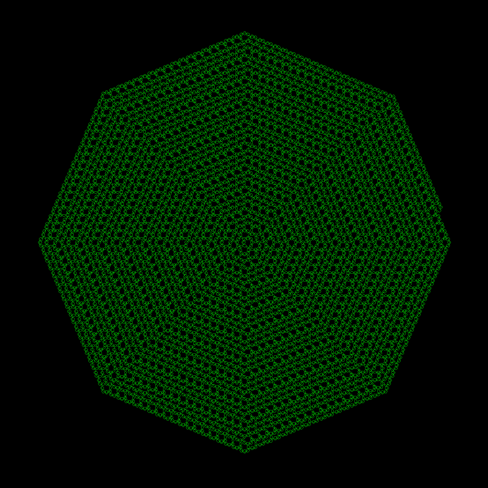
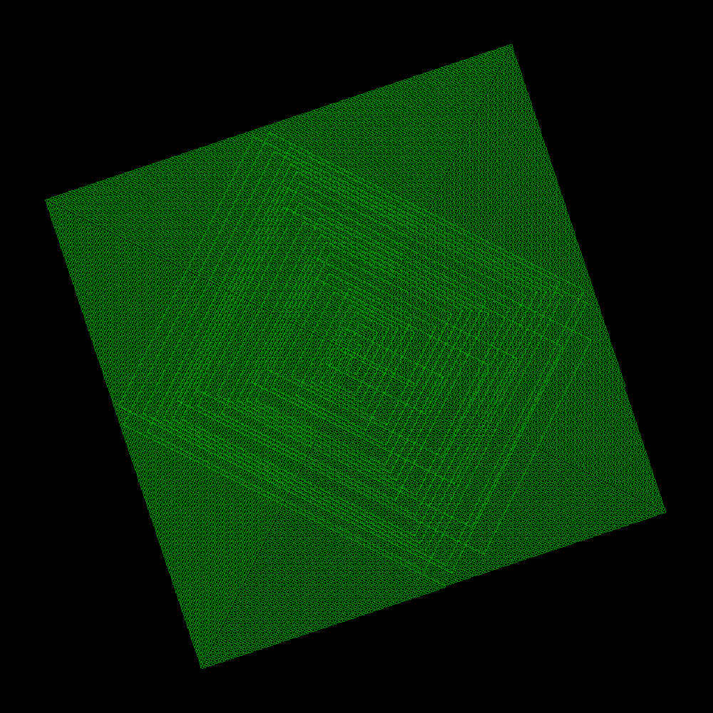
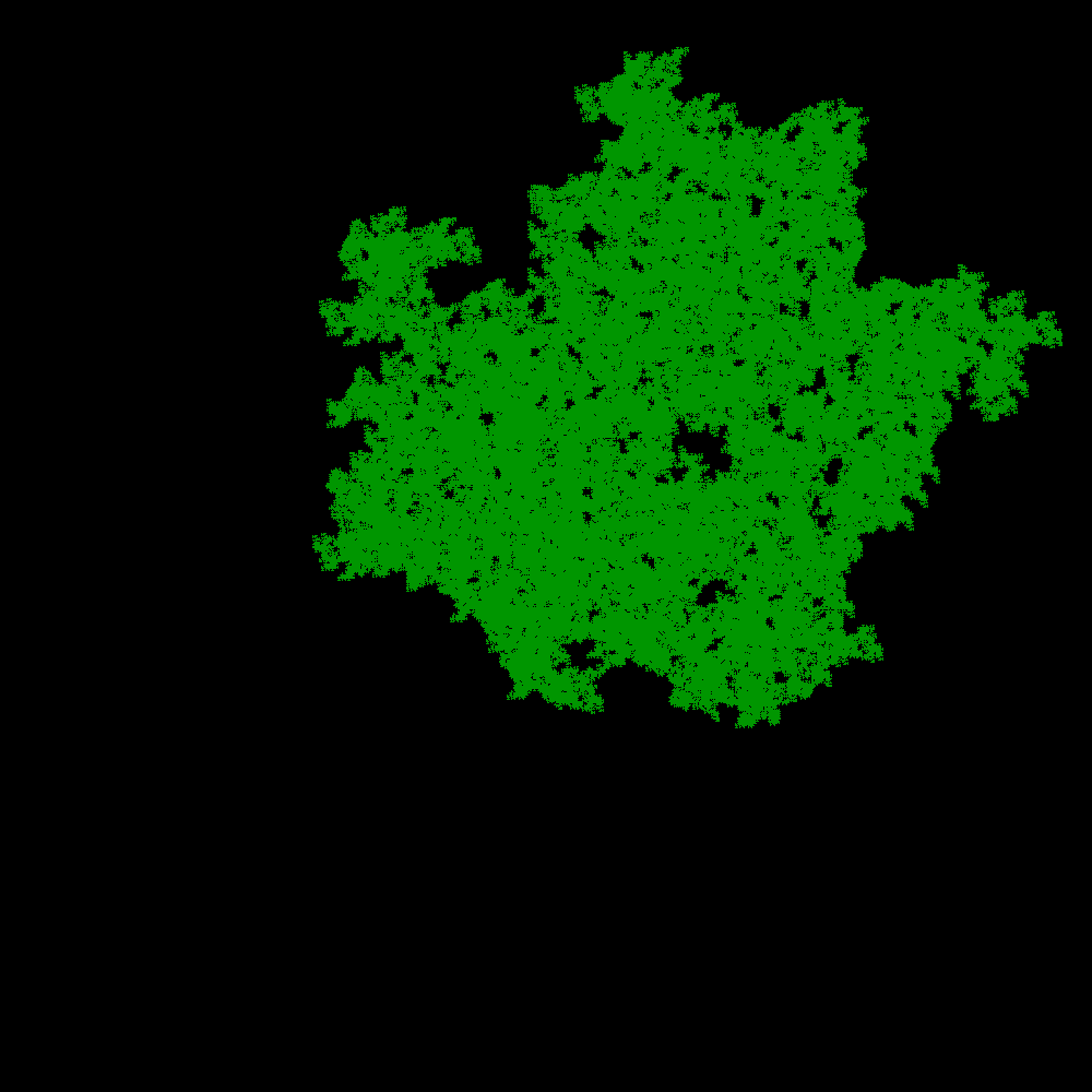
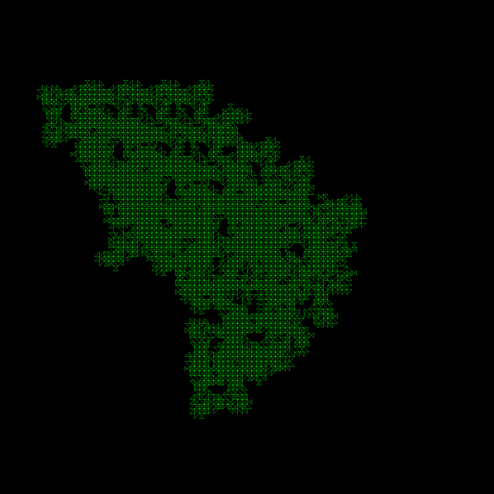
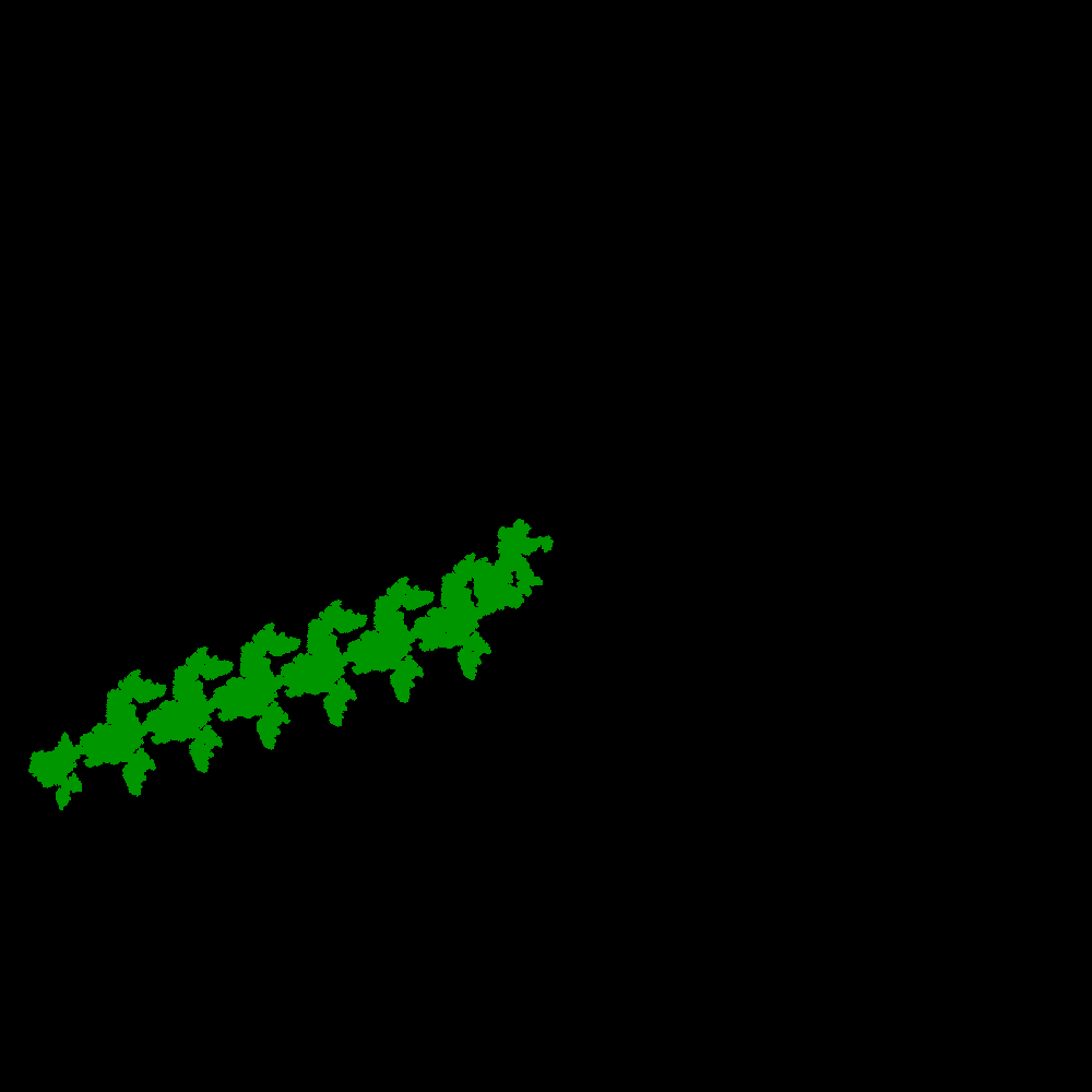
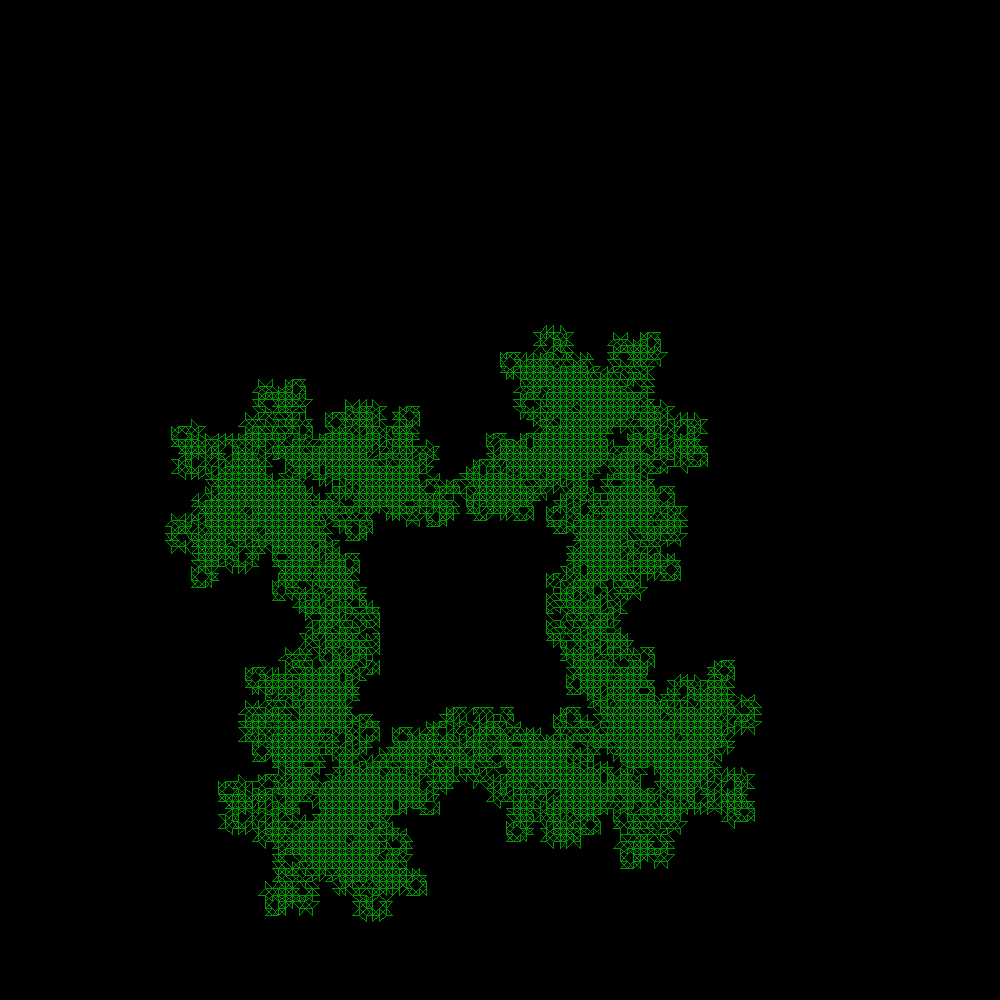
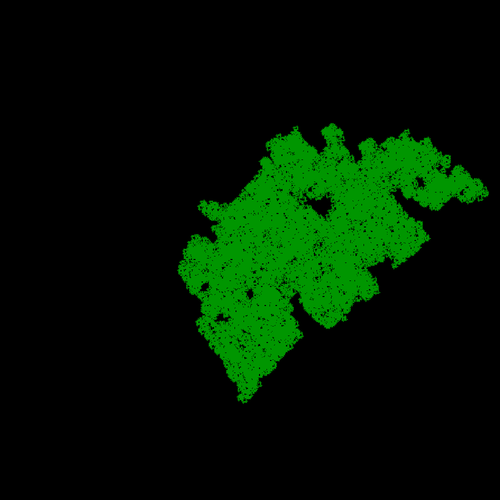
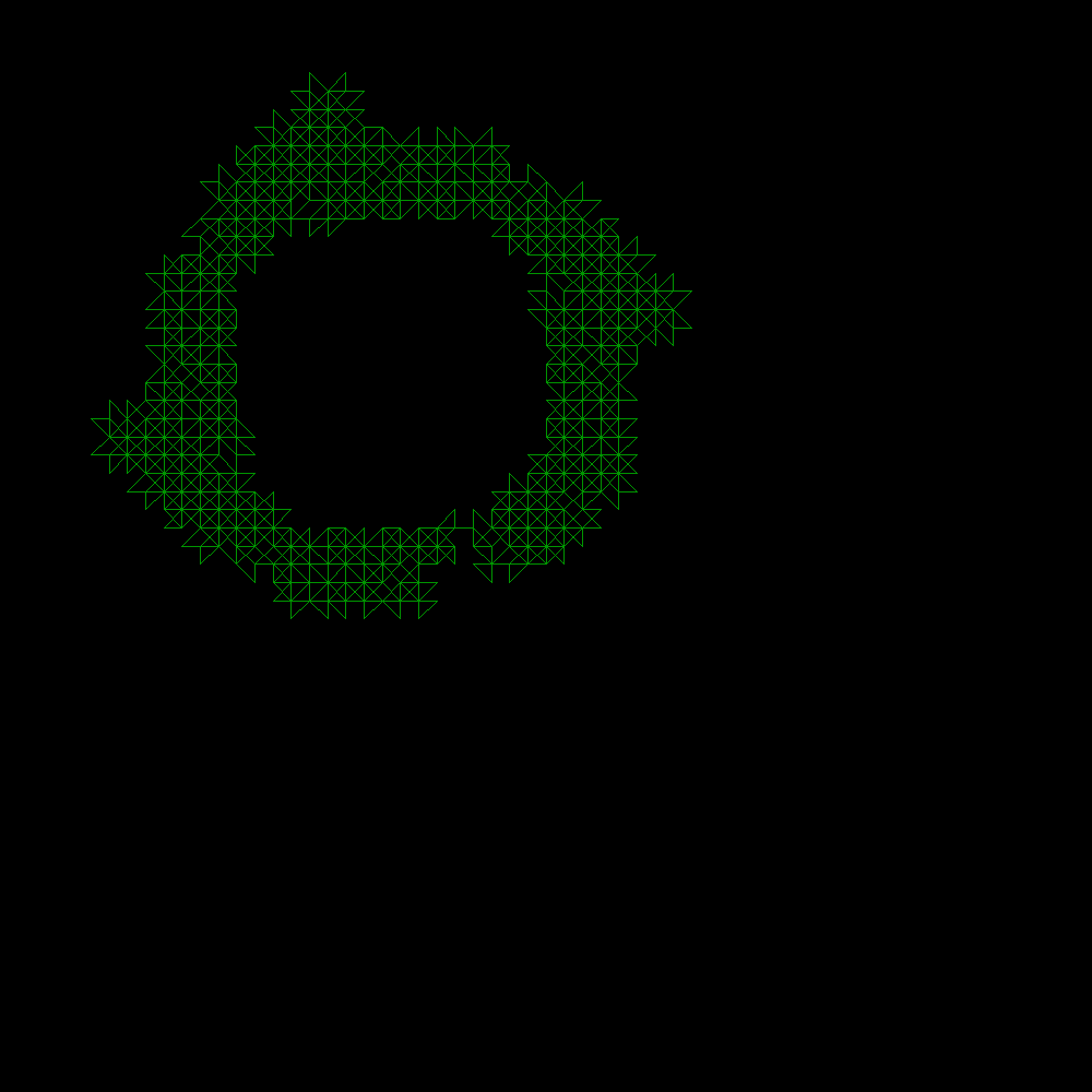
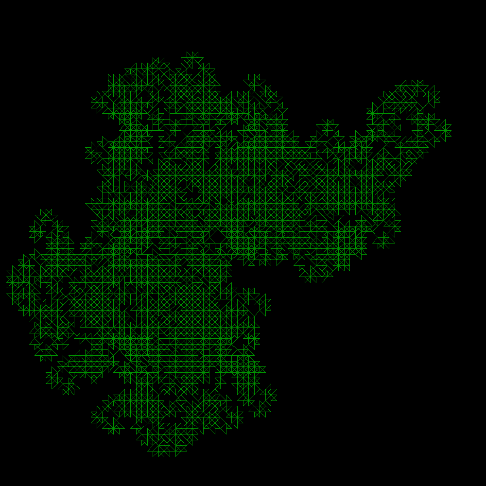
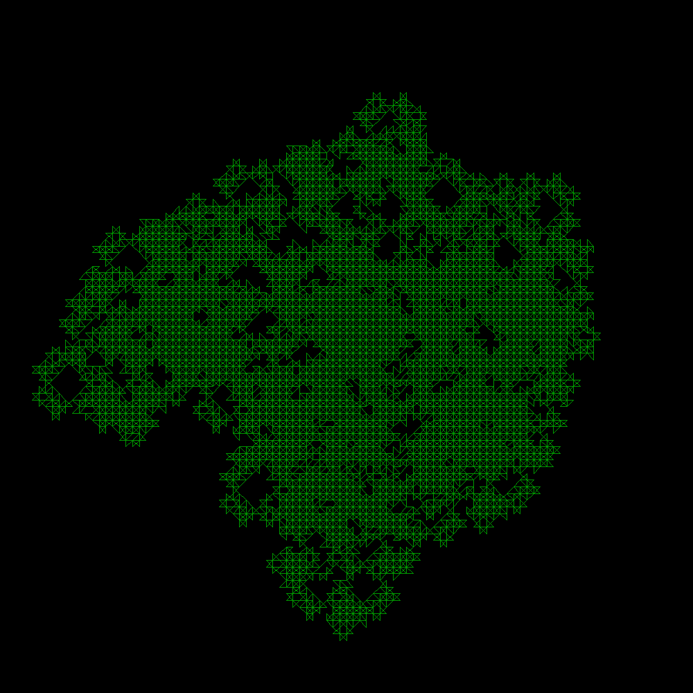
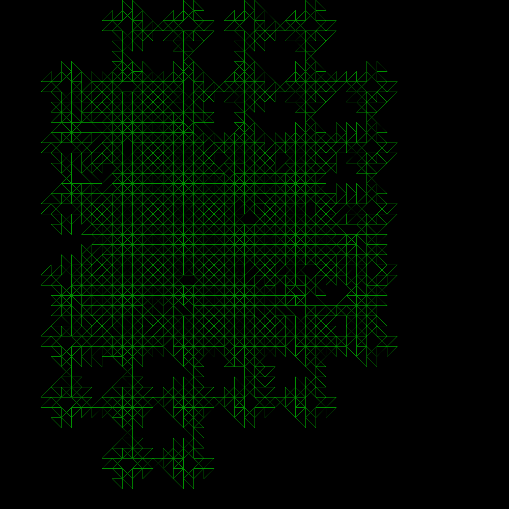
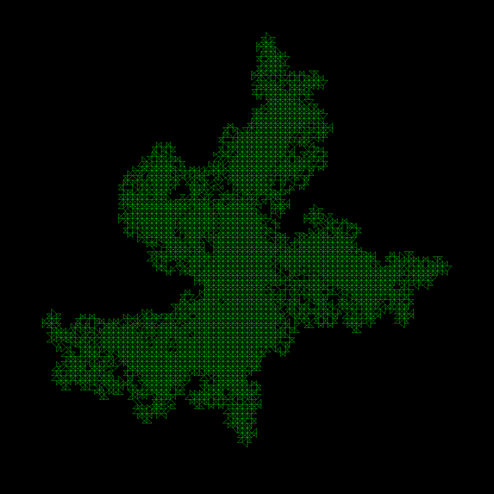
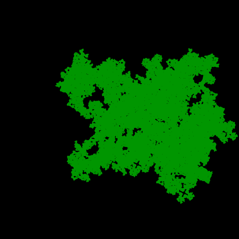
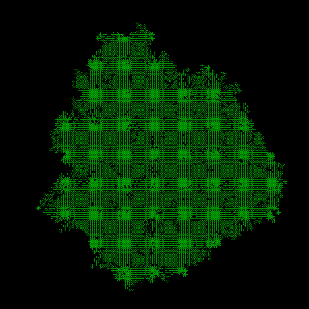
Some examples of the resulting worm patterns are available to view here.
An interactive evolutionary computation (IEC) model is available to view the entire set of unique worms as a tree including branch nodes to a depth of 5 rules.
Currently there are many worms for which the outcome remains unknown, running beyond 12 million population. To see some examples of those worms remaining in category R in higher resolution detail, click here
The definitive full results table shows pictures of all unique worms to depth of 5 rules, and lists the status, population size, worm category, number of rules, loop sizes and other details, for every worm, on this results page.
The Evolutionary History page shows the full parantage of every worm in a family tree with up to 5 generations per worm, so that the evolutionary changes between the worm species can be visualised.
The 8 path worm code has been ported into a free JavaScript Web browser compatible version which has been developed and tested. This allows all worms to be modelled in real-time on any web browser. This supports many web browsers and platforms including: Windows, Internet Explorer, Edge, Apple, Safari, Firefox, Google Chrome, and Android browsers.
A compiled windows .exe file for 64 bit computers can be downloaded here. This is a faster ANSI C program to run large worms up to maximum of 12 million population.
References
[1] Rasmussen, B., Bengtson, S., Fletcher, I. R., & McNaughton, N. J. (2002). Discoidal impressions and trace-like fossils more than 1200 million years old. Science, 296(5570), 1112-1115.
[2] Raup. D., (1969), Fossil Foraging Behavior: Computer Simulation, Science, Vol 166, https://sci-hub.tf/10.1126/science.166.3908.994
[3] Seilacher, A. (1967). Fossil behavior. Scientific American, 217(2), 72-83.
[4] Prescott, T, Ibbotson C. 1997. A robot trace maker: Modeling the fossil evidence of early invertebrate behavior. Artificial Life 3:289-306.
[5] Kahrkling S, (2004), Pattern Inventory, (Online, Accessed 12th May 2022) https://web.archive.org/web/20040428090952/http://www.accessv.com/~sven/worms/wo04.htm
[6] Beeler M, (1973) Paterson’s Worm, MIT AI Laboratory, Memo No. 290. http://hdl.handle.net/1721.1/6210
[7] Gardner M (1973) Fantastic patterns traced by programmed "worms", Scientific American, Mathematical Games column, November 1973 issue.
[8] Pegg Jr, E. (2003), Paterson's Worms Revisited https://web.archive.org/web/20040323220627/http://www.maa.org/editorial/mathgames/mathgames_10_24_03.html
[9] Rokicki T, (2003), Algorithm based on Hashlife, https://web.archive.org/web/20031204221203/http://tomas.rokicki.com/worms.html
[10] Chaffin B, (2004), Paterson’s Worms https://web.archive.org/web/20040420235026/http://wso.williams.edu/~bchaffin/patersons_worms/index.htm
[11] Hayes, B. (2003). Computing Science: In Search of the Optimal Scumsucking Bottomfeeder. American Scientist, 91(5), 392-396
[12] Vaughan N (2022), Digital worm simulation path traces https://empslocal.ex.ac.uk/people/staff/nv266/worm.htm
[13] Kahrkling S (2022), http://scientific601.altervista.org/patersonswormsprogram.html
8 path worms © Neil Vaughan 2021, University of Exeter.