| Independent Component Analysis |
|
|
|
|
| RME Home |
| DCS Home |
| Research |
| Teaching |
| Publications |
| Contact |
|
|
| Email me |

Finding a natural coordinate system for empirical data is an essential first step in its analysis. Principal components analysis (PCA) is often used to find a basis set which is determined by the dataset itself. The principal components are orthogonal and projections of the data onto them are linearly decorrelated, which can be ensured by considering the second order statistical properties of the data. Independent components analysis (ICA), which has enjoyed recent theoretical and empirical attention, aims at a loftier goal: it seeks a linear transformation (an unmixing matrix) to coordinates in which the data are maximally statistically independent, not merely decorrelated. Statistical independence is measured by the mutual information between the unmixed variables and ICA algorithms seek unmixing matrices which minimise the mutual information. Viewed from another perspective, ICA is a method of separating independent sources, which have been linearly mixed to produce the data.
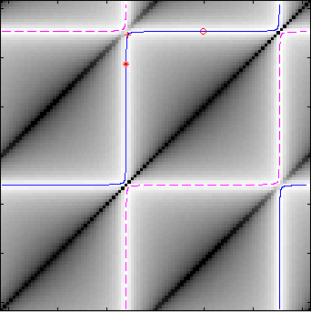
Decorrelating manifold
It is useful to consider ICA in terms of the likelihood of the unmixing matrix having produced the data. Cardoso and MacKay have each shown that the maximum likelihood unmixing matrix is the matrix found by Bell and Sejnowski's infomax algorithm.
An unmixing matrix which finds independent components must also decorrelate those components. Consequently the ICA unmixing matrix must lie on the manifold of decorrelating matrices, and this leads to efficient algorithms for finding the ICA transformation.
The picture shows the manifold of (row-normalised) decorrelating matrices plotted on the likelihood function for a mixture of Gaussian and Laplacian (bi-exponential) sources. Up to a scaling, which does not affect the mutual information, two-dimensional unmixing matrices are parameterised by two angles. The gray scale shows the likelihood at each point shows the likelihood of the unmixing matrix parameterised by the angles on the abscissa and ordinate. The decorrelating manifold, which consists of two leaves, is plotted as blue and magenta lines,corresponding to unmixing matrices positive and negative determinant. The symbols mark the locations of decorrelating matrices corresponding to PCA (circle), zero-phase components analysis (+) and ICA (*).
For more on this and some other aspects of ICA read ICA: A flexible non-linearity and decorrelating manifold approach.
Learning the nonlinearity
Most ICA algorithms implicitly assume a particular form for the marginal probability densities of the unmixed variables (see our paper where we elucidate how ICA algorithms using static nonlinearities cope with sources with differing marginal densities.) A common feature of these algorithms is that they can separate heavy tailed densities but not those with tails lighter than Gaussian, such as uniform densities. We have used generalised exponentials to model the marginal densities and our algorithm is able to separate a mixture of heavy and light tailed sources.
Demonstration
As a demonstration we mix three sources: uniform noise and two fragments of music (part of Beethoven's String Quartet in C major Op59, number 3 and the blues ballad "Baby won't you please come home", sung by Bessie Smith on an old and noisy recording). The three mixed channels are here: mix1, mix2, mix3.
Many ICA algorithms are unable to separate the light tailed uniform noise from the Beethoven and ballad. Using generalised exponentials we are able to almost perfectly separate the sources. unmix1, unmix2, unmix3. In particular there is no trace of music in the unmixed noise variable.
Graphs and more details are given in A flexible non-linearity and decorrelating manifold approach to ICA.