Time series components

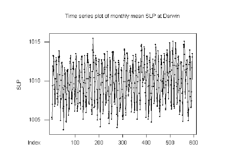
A lot can be learnt about a time series by plotting $x_k$ versus $t_k$ in a time series plot. For example, the time series plot in Figure 9.1 shows the evolution of monthly mean sea-level pressures measured at Darwin in northern Australia.

Figure: Time series of the montly mean sea-level pressure observed at Darwin in northern Australia over the period January 1950 to July 2000.

A rich variety of structures can be seen in the series that include:

• Trends - long-term changes in the mean level. In other words, a smooth regular component consisting primarily of Fourier modes having periods longer than the length of the time series. Trends can be either deterministic (e.g. world population) or stochastic. Stochastic trends are not necessarily monotonic and can go up and down (e.g. North Atlantic Oscillation). Extreme care should be exercised in extrapolating trends and it is wise to always refer to them in the past tense.

• (Quasi-)periodic signals - having clearly marked cycles such as the seasonal component (annual cycle) and interannual phenomena such as El Niño and business cycles. For periodicities approaching the length of the time series, it becomes extremely difficult to discriminate these from stochastic trends.

• Irregular component - random or chaotic noisy residuals left over after removing all trends and (quasi-)periodic components. They are (second-order) stationary if they have mean level and variance that remain constant in time and can often be modelled as filtered noise using time series models such as ARIMA.

Some time series are best represented as sums of these components (additive) while others are best represented as products of these components (multiplicative). Multiplicative series can quite often be made additive by normalizing using the logarithm transformation (e.g. commodity prices).