ARIMA(p,d,q) time series models

Auto-Regressive Integrated Moving Average (ARIMA) time series models form a general class of linear models that are widely used in modelling and forecasting time series (Box and Jenkins, 1976). The ARIMA(p,d,q) model of the time series $\{x_1,x_2,\ldots\}$ is defined as

$$\Phi_p(B)\Delta^d x_t = \Theta_q(B)\epsilon_t$$ (9.4)

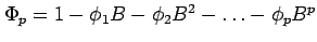
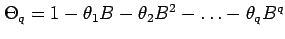
where $B$ is the backward shift operator, $Bx_y=x_{y-1}$, $\Delta=1-B$ is the backward difference, and $\Phi_p$ and $\Theta_q$ are polynomials of order $p$ and $q$, respectively. ARIMA(p,d,q) models are the product of an autoregressive part AR(p) $\Phi_p=1-\phi_1B-\phi_2B^2-\ldots-\phi_pB^p$, an integrating part $I(d)=\Delta^{-d}$, and a moving average MA(q) part $\Theta_q=1-\theta_1B-\theta_2B^2-\ldots-\theta_qB^q$. The parameters in $\Phi$ and $\Theta$ are chosen so that the zeros of both polynomials lie outside the unit circle in order to avoid generating unbounded processes. The difference operator takes care of ``unit root'' $(1-B)$ behaviour in the time series and for $d>0.5$ produces non-stationary behaviour (e.g. increasing variance for longer time series).

An example of an ARIMA model is provided by the ARIMA(1,0,0) first order autoregressive model 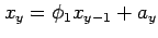$x_y=\phi_1 x_{y-1}+a_y$. This simple AR(1) model has often been used as a simple ``red noise'' model for natural climate variability.