Serial correlation

Successive values in time series are often correlated with one another. This persistence is known as serial correlation and leads to increased spectral power at lower frequencies (redness). It needs to be taken into account when testing significance, for example, of the correlation between two time series. Among other things, serial correlation (and trends) can severely reduce the effective number of degrees of freedom in a time series. Serial correlation can be explored by estimating the sample autocorrelation coefficients

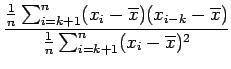$$r_k = \frac{\frac{1}{n} \sum_{i=k+1}^{n}(x_i-\overline{x})(x_{i-k}-\overline{x})}{\frac{1}{n} \sum_{i=k+1}^{n}(x_i-\overline{x})^2}$$ (9.3)

where $k=0,1,2,\ldots$ is the time lag. The zero lag coefficient $r_0$ is always equal to one by definition, and higher lag coefficients generally damp towards small values with increasing lag. Only autocorrelation coefficients with lags less than $n/4$ are sufficiently well-sampled to be worth investigation.

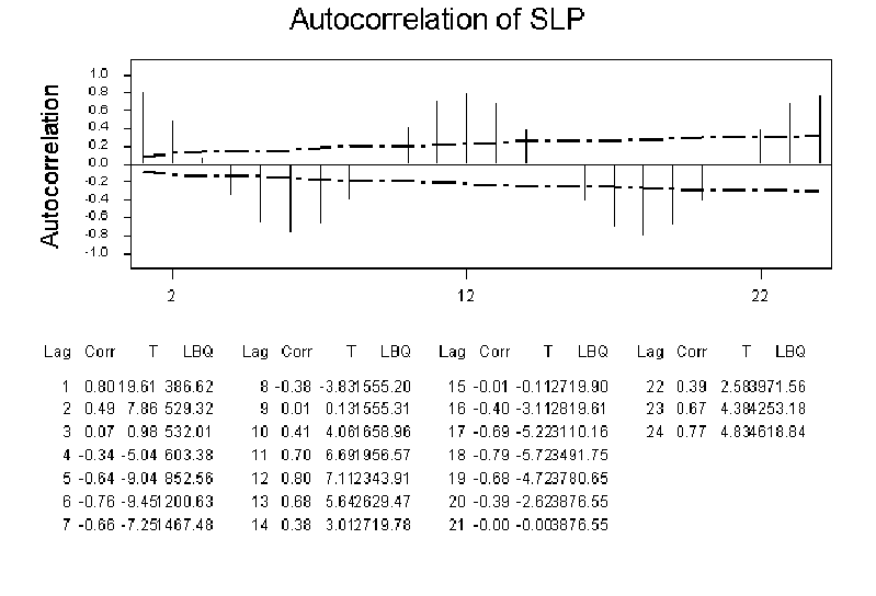
The autocorrelation coefficients can be plotted versus lag in a plot known as a correlogram. The correlogram for the Darwin series is shown in Fig. 9.3. Note the fast drop off in the autocorrelation function (a.c.f.) for time lags greater than 12 months. The lag-1 coefficient is often (but not always) adequate for giving a rough indication of the amount of serial correlation in a series. A rough estimate of the decorrelation time is given by $\tau_0=-\tau/\log(r_1)$ and the effective number of degrees of freedom is given by $n\tau/\tau_0=-n\log(r_1)$. See von Storch and Zwiers (1999) for more details.

Figure: Correlogram showing the autocorrelations as a function of lag for the Darwin series