It is a reasonable hypothesis to expect that body height
may be an important factor in determining the body weight
of a Reading meteorologist.
This dependence is apparent in the scatter plot below
showing the paired weight versus height data ![]() for the sample of meteorologists at Reading. Scatter plots are useful ways
of seeing if there is any relationship between multiple variables and
should always be performed before quoting summary measures of linear
association such as correlation.
for the sample of meteorologists at Reading. Scatter plots are useful ways
of seeing if there is any relationship between multiple variables and
should always be performed before quoting summary measures of linear
association such as correlation.
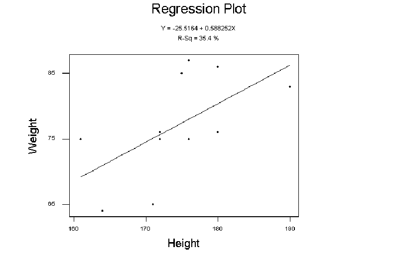 |
The response variable (weight) is plotted along the y-axis while the explanatory variable (height) is plotted along the x-axis. Deciding which variables are responses and which variables are explanatory factors is not always easy in interacting systems such as the climate. However, it is an important first step in formulating the problem in a testable (model-based) manner. The explanatory variables are assumed to be error-free and so ideally should be control variables that are determined to high precision.
The cloud of points in a scatter plot can often (but not always!) be imagined to lie inside an ellipse oriented at a certain angle to the x-axis. Mathematically, the simplest description of the points is provided by the additive linear regression model
| (7.1) |
where ![]() are the values of the response variable,
are the values of the response variable, ![]() are
the values of the explanatory variable, and
are
the values of the explanatory variable, and
![]() are
the left-over noisy residuals caused by random effects
not explainable by the explanatory variable. It is normally assumed
that the residuals
are
the left-over noisy residuals caused by random effects
not explainable by the explanatory variable. It is normally assumed
that the residuals
![]() are uncorrelated Gaussian
noise, or to be more precise, a sample of independent and
identically distributed (i.i.d.) normal variates.
are uncorrelated Gaussian
noise, or to be more precise, a sample of independent and
identically distributed (i.i.d.) normal variates.
Equation 7.1 can be equivalently expressed as the following
probability model:
| (7.2) |
The model parameters ![]() and
and ![]() are the y-intercept
and the slope of the linear fit, and
are the y-intercept
and the slope of the linear fit, and
![]() is the standard
deviation of the noise. These three parameters can be estimated
using least squares by minimising the sum of squared residuals
is the standard
deviation of the noise. These three parameters can be estimated
using least squares by minimising the sum of squared residuals
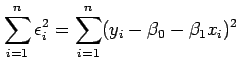 |
(7.3) |
By solving the two simultaneous equations
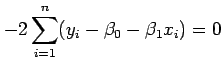 |
(7.4) | ||
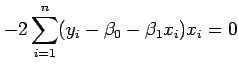 |
(7.5) |
it is possible to obtain the following least squares estimates
of the two model parameters:
| (7.6) | |||
| (7.7) |
Since the simultaneous equations involve only first and second moments of the variables, least squares linear regression is based solely on knowledge of means and (co)variances. It gives no information about higher moments of the distribution such as skewness or the presence of extremes.