When MINITAB is used to perform the linear regression of weight on height it gives the following results:
The regression equation is
Weight = - 25.5 + 0.588 Height


Predictor       Coef    StDev       T       P
Constant        -25.52  46.19   -0.55   0.594
Height          0.5883 0.2648    2.22   0.053

S = 6.606       R-Sq = 35.4%     R-Sq(adj) = 28.2%

Analysis of Variance

Source          DF      SS      MS      F       P
Regression       1      215.30  215.30  4.93    0.053
Residual Error   9      392.70   43.63
Total           10      608.00
The regression equation
![]() is the equation of the straight line
that ``best'' fits the data.
The hat symbol
is the equation of the straight line
that ``best'' fits the data.
The hat symbol ![]() is used to denote ``predicted (or estimated) value''.
Note that regression is not symmetric: a regression of x on y does not
generally give the same relationship to that obtained from regression
of y on x.
is used to denote ``predicted (or estimated) value''.
Note that regression is not symmetric: a regression of x on y does not
generally give the same relationship to that obtained from regression
of y on x.
The Coef column gives the best estimates of the model parameters
associated with the explanatory variables
and the StDev column gives an estimate of
the standard errors in these estimates. The standard error on
the slope is given by
 |
(7.8) |
The other two columns can be used to assess the statistical significance of the parameter estimates. The T column gives the ratio of the parameter estimate and its standard error whereas the P column gives a p-value (probability value) for rejection of the null hypothesis that the parameter is zero (i.e. not a significant linear factor). For example, a p-value of 0.05 means that there is 5% chance of finding data less consistent with the null hypothesis (zero slope parameter) than the fitted data. Small p-values mean that it is unlikely that the slope was non-zero purely by chance.
The overall goodness of fit can be summarised by calculating the
fraction of total variance explained by the fit
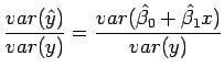 |
(7.9) |
The MINITAB output contains an ANalysis Of VAriance (ANOVA) table
in which the sums of squares SS equal to ![]() times the variance
are presented for the regression fit
times the variance
are presented for the regression fit ![]() ,
the residuals
,
the residuals ![]() , and the total response
, and the total response ![]() .
ANOVA can be used to test the significance of the fit by applying
F-tests on the ratio of variances. The p-value in the ANOVA table
gives the statistical significance of the fit.
When summarizing a linear regression, it is important to quote
BOTH the coefficient of determination AND the p-value. With
the small sample sizes often encountered in climate studies,
fits can have substantial
.
ANOVA can be used to test the significance of the fit by applying
F-tests on the ratio of variances. The p-value in the ANOVA table
gives the statistical significance of the fit.
When summarizing a linear regression, it is important to quote
BOTH the coefficient of determination AND the p-value. With
the small sample sizes often encountered in climate studies,
fits can have substantial ![]() values yet can still fail
to be significant (i.e. do not have a small p-value).
values yet can still fail
to be significant (i.e. do not have a small p-value).