Model fit validation using residual diagnostics

In addition to the basic summary statistics above, much can be learned about the validity of the model fit by examining the left-over residuals. The linear model is based on certain assumptions about the noise term (i.e. independent and Gaussian) that should always be tested by examining the standardized residuals. Resisduals should be tested for:

1. Structure The standardized residuals should be identically distributed with no obvious outliers. To check this, plot $\epsilon_i$ versus $i$ and look for signs of structure. The residuals should appear to be randomly scattered (normally distributed) about zero.

   Figure: Residuals versus order of points for the regression of weight on height.

   

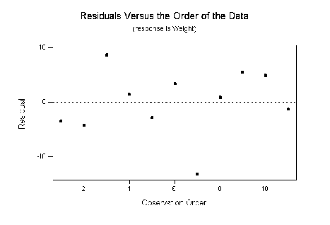2. Independence The residuals should be independent of one another. For example, there should be no sign of runs of similar residuals in the plot of $\epsilon_i$ versus $i$. Autocorrelation functions should be calculated for regularly spaced residuals to test that the residuals are not serially correlated.

3. Outliers There should not be many standardised residuals with magnitudes greater than 3. Outlier points having large residuals should be examined in more detail to ascertain why the fit was so poor at such points.

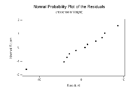
4. Normality The residuals should be normally distributed. This can be examined by plotting a histogram of the residuals. It can be tested by making a normal probability plot in which the normal scores of the residuals are plotted against the residual value. Straight line indicates normal distribution.

   Figure: Normal probability plot of the residuals for the regression of weight on height.

   

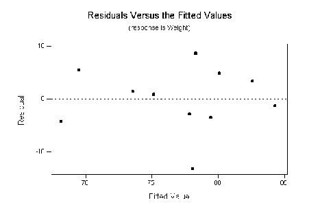
5. Linearity The residuals should be independent of the fitted (predicted) values $\{\hat{y_i}\}$. This can be examined by making a scatter plot of $\epsilon_i$ versus $\{\hat{y_i}\}$. Lack of uniform scatter suggests that there may be a nonlinear dependence between $y$ and $x$ that could be better modelled by transforming the variables. For mutliple regression, with more than one explanatory variable, the residuals should be independent of ALL the explanatory variables.

   Figure: Residuals versus the fitted values for the regression of weight on height.

   

In addition to these checks on residuals, it is also important to check whether the fit has been dominated by only a few influential observations far from the main crowd of points that can have high leverage. The leverage of a particular point can be assessed by testing the mean squared differences of all the predicted values to leaving out this point (known as Cook's distances).