
| Cortical layout |
|
|
|
|
| RME Home |
| DCS Home |
| Research |
| Teaching |
| Publications |
| Contact |
|
|
| Email me |
The long term goal is to understand the principles underlying the functional architecture of the cortex. Experiments on the visual cortex have revealed a rich organizational structure: most cortical areas possess a visuotopic map, and neurons subserving various modes of cortical response are commonly clustered together. Experiments alone, however, cannot determine the principles which govern the layout of the cortex. Thus there is a need to model the function of cortical areas and the constraints upon it. The essential function of a neuron in the visual cortex is to compare and correlate its inputs with those of other cortical neurons. Resources available to the cortex are scarce and interconnections demanded by the functionality are expensive: long connections are metabolically expensive, they slow down communication, and they reduce the cortical volume available for the neurons themselves.
This work aims to test the hypothesis that the cortical architecture of specific visual areas is determined by a balance between the functions that a cortical neuron must perform (comparing and correlating inputs) and the cost of making and maintaining the intra-cortical connections.
What is the function of a cortical neuron? In a general sense, it must compare or correlate inputs from many positions in visual space. To accomplish this it must be wired to many other neurons. Clearly, a cortical neuron cannot be wired to every other neuron. However, it is most important for it to be connected to neurons that are looking at neighboring regions of visual space. Given this requirement, we can ask: what is the best way to arrange neurons on a laminar cortex so as to minimize the wiring cost?
We define a metric of the architectural efficiency of a particular layout. The metric then equips us to
- Evaluate the efficiency of a particular (perhaps experimentally measured) layout.
- Rearrange to locations of neurons on a fictitious, computational cortex in order to find the most efficient arrangement.
Retinotopic map
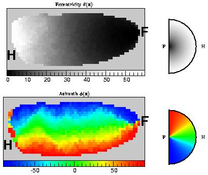
The figure shows a simulation of the visuotopic map of macaque V1. The computational "V1" is approximately the shape of flattened macaque V1. The shows the optimum configuration of cortical neurons found after simulated annealing from a random initial configuration. The left panel is a map of the eccentricity of each cortical neuron's receptive field (shown as a gray scale), and the bottom panel shows the azimuthal angle on a color scale. Thus the receptive field location of a particular computational "neuron" is obtained by reading the eccentricity from the top panel and the azimuthal angle from the bottom panel. Neurons shaded dark gray have receptive fields lying close to the fovea, while those drawn in white look at peripheral regions out to about 70 degrees. The amount of cortex devoted to foveal regions is apparent from the amount of dark gray in the picture. The distribution of eccentricities was chosen so that the cortical magnification factor obeys the measured form.
The position of the foveal representation (F), at the far left hand of V1 is in the right place, as is the approximate location of the horizontal meridian, which ends at H on the far right. In common with real V1, the peripheral regions of the hemifield are represented around the edges of the computational V1. It should also be noted that the map is smooth. Although this was not built into the mode: it would have been possible for the map to have been discontinuous. In the optimum configuration neurons with nearby receptive fields are placed close together, and it is efficient to place neurons with distant receptive fields far apart on the cortex. The inefficiency for this optimized layout was 323, compared with 630 for the mean of 10 random configurations.
Orientation pinwheels
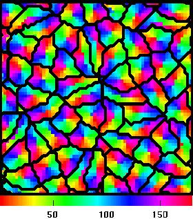
This picture shows the result of a simulation of a small patch of cortex whose neurons are selective for orientation as well as having different receptive field locations.
The computation, which started from a random configuration of cortical neurons, involved 8 x 8 "retinal neurons" which projected to 64 x 64 "cortical neurons". The picture shows the orientation preference (between 0 and 180 degrees) of the neuron at each location. The orientation map is not as regular as experimentally observed configurations, but it consists of pinwheels. The superimposed black lines delineate regions in which the receptive field locations are similar. In each of these regions the orientation preferences are arranged as a single pinwheel, so they might be regarded as the analogues of hypercolumns, since each one contains the necessary machinery to process the full range of orientations for a particular point in visual space.
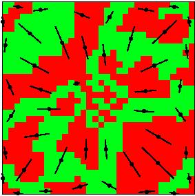
Ocular dominance columns and cortical shear
When the visuotopic map is uniform small circles in visual space are represented by small circles on the cortex. In general, however, the visuotopic map is not completely isotropic and transforms small circles in visual space into ellipses on the cortex. The major axes of the ellipses define the local directions in which the visuotopic map is most stretched.
Recent optical imaging measurements by Blasdel suggest that the boundaries of ocular dominance columns in monkeys run perpendicular to this direction of maximum stretch.
In order to investigate this effect, an optimisation calculation was performed in which the distribution of receptive fields was set up so that the visuotopic map would be anisotropic. The final configuration is shown in the picture. Red and green code neurons responding to left and right eye stimulation. The direction and magnitude of maximum stretch in the visuotopic map for the final configuration was calculated, and is shown by orientation and length of the black and red lines. In the optimised layout the ocular dominance column boundaries are approximately perpendicular to the stretch in the retinotopic map. Although the simulation is crude it concurs qualitatively with Blasdel's measurements and suggests an explanation for the phenomenon.
Young and Scannell give an interesting review of instances in which biological wiring length is not minimised.