The prediction of quasi-Brownian behaviour made in the previous
section could be verified within the limits of the model system, in the
style of [9] or [13]. This, however, would be
essentially a numerical check of rigorously proved statements, and so
it is more interesting to observe this type of behaviour in a
particular reaction-diffusion system. There are a few papers in which
hypermeandering spiral waves were reported; not all of them were we
able to reproduce. So, the cubic FitzHugh-Nagumo model with
parameters reported in [7] as providing a hypermeander,
did show a rather complicated behaviour, -- however, in our
experiments this complicated behaviour only lasted a few dozens of
spiral revolutions, whereafter standard flower-like meander
established. The Oregonator model with parameters described in
[8] showed complicated and obviously not flower-like tip
trajectory. However, that trajectory remained compact for the longest
time scales we followed it (up to ![]() t.u.), which,
apparently, means that the quotient system had complicated but not
chaotic dynamics. This is consistent with observations of Plesser &
Müller [15] of up to four-periodic motions and no chaos in
Oregonator spiral waves.
t.u.), which,
apparently, means that the quotient system had complicated but not
chaotic dynamics. This is consistent with observations of Plesser &
Müller [15] of up to four-periodic motions and no chaos in
Oregonator spiral waves.
Eventually, we have chosen Barkley's model [16] for our experiments:
for two reasons. First, it is fastest for simulation, which is provided
by the efficient numeric algorithm of [16]. This
algorithm, in particular, includes resetting ![]() to the null-cline
value 0 or 1 if it becomes too close (closer than
to the null-cline
value 0 or 1 if it becomes too close (closer than ![]() ) to
one of them, so that in a large number of nodes there is no need to
compute Laplacian which is zero. Second, we were able to find parameter
values which produced intensive and persistent hypermeander with
clearly nonlocal tip trajectory:
) to
one of them, so that in a large number of nodes there is no need to
compute Laplacian which is zero. Second, we were able to find parameter
values which produced intensive and persistent hypermeander with
clearly nonlocal tip trajectory:
Both these aspects are crucial, as the statistical predictions of the
Theorem required very long experiments. The grid steps were chosen
![]() s.u. in space and
s.u. in space and ![]() t.u. in time. The time step is
small enough to obey diffusion stability criterion
t.u. in time. The time step is
small enough to obey diffusion stability criterion ![]() , but
since
, but
since ![]() , local kinetics of
, local kinetics of ![]() variable were
calculated using implicit version of [16]. This choice
of computation steps is rather far from giving a fully resolved PDE
simulation, -- however, the major approximation error produced by the
implicit calculation of fast local kinetics of
variable were
calculated using implicit version of [16]. This choice
of computation steps is rather far from giving a fully resolved PDE
simulation, -- however, the major approximation error produced by the
implicit calculation of fast local kinetics of ![]() , did not influence
the symmetry of the model, and change of the dynamic field in one time
step always remained small. So, we believe that the computational model
used is of a spatially extended dynamical system with all the required
symmetry properties, and is suitable for testing the theory considered,
no matter what its exact relation to the PDE system
(21).
, did not influence
the symmetry of the model, and change of the dynamic field in one time
step always remained small. So, we believe that the computational model
used is of a spatially extended dynamical system with all the required
symmetry properties, and is suitable for testing the theory considered,
no matter what its exact relation to the PDE system
(21).
Maximal medium size was ![]() s.u., i.e.
s.u., i.e. ![]() grid
nodes. The spiral wave was initiated from cross-gradient initial
conditions:
grid
nodes. The spiral wave was initiated from cross-gradient initial
conditions: ![]() was assigned to 0 in the left half of the medium and
to 1 in the right half, and
was assigned to 0 in the left half of the medium and
to 1 in the right half, and ![]() was assigned to 0 in the bottom
half of the medium and to a/2 in the upper half. The spiral wave and
typical tip trajectory are illustrated in Fig. 1.
was assigned to 0 in the bottom
half of the medium and to a/2 in the upper half. The spiral wave and
typical tip trajectory are illustrated in Fig. 1.
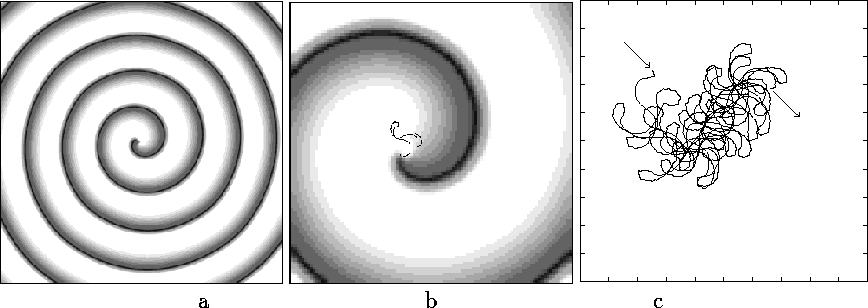
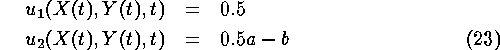
Figure 1:
(a) Spiral wave in the medium ![]() s.u. large. Darkness of
shading shows sum of the values of activator variable
s.u. large. Darkness of
shading shows sum of the values of activator variable ![]() and
inhibitor variable
and
inhibitor variable ![]() .
(b) Same, in the medium
.
(b) Same, in the medium ![]() s.u. The black line is a piece of
trajectory of the tip.
(c) Piece of the tip trajectory during 40 t.u.; arrows show begin and
end of the piece, size of the square is
s.u. The black line is a piece of
trajectory of the tip.
(c) Piece of the tip trajectory during 40 t.u.; arrows show begin and
end of the piece, size of the square is ![]() s.u., cut from the
medium
s.u., cut from the
medium ![]() s.u.
s.u.
This shows that the trajectory looks evidently more complicated than
regular `flowers' of simple meander, thus it may be called
hypermeander. To see evolution of the tip at long times, we used
histograms of tip position, obtained with bins of ![]() grid
cells (see Fig. 2). This solution was followed for about
grid
cells (see Fig. 2). This solution was followed for about
![]() time steps, or
time steps, or ![]() t.u., when the spiral
wave has died out by reaching the boundary.
t.u., when the spiral
wave has died out by reaching the boundary.
Figure 2:
Histogram of the tip position, (a) through the first 800 t.u., (b)
through the whole duration of numerical experiment, ![]() t.u.
Medium size
t.u.
Medium size ![]() s.u. The peak at the far border of panel (b)
corresponds to the tip attaching the boundary before dying out.
s.u. The peak at the far border of panel (b)
corresponds to the tip attaching the boundary before dying out.
It can be seen in that figure, that the tip does walk in the plane to large distances. We have found that this trajectory is long enough to interpret the behaviour of this system in terms of the proposed theory.
To do that, we extracted tip path data X(t), Y(t) and ![]() ,
where X and Y were coordinates of the crossing of two isolines,
,
where X and Y were coordinates of the crossing of two isolines,
and ![]() was
the azimuthal angle of
was
the azimuthal angle of ![]() calculated at the tip point,
calculated at the tip point,
The gradient has been calculated by central differences at the corners of the computational cell containing the tip, and then bilinearly interpolated to the tip point.
The time derivatives ![]() ,
, ![]() and
and ![]() were
substituted into (3,4) to reconstruct
were
substituted into (3,4) to reconstruct ![]() and
and
![]() . The numerical differentiation was performed with simplest
Tikhonov regularisation procedure [17] with regularising
functional
. The numerical differentiation was performed with simplest
Tikhonov regularisation procedure [17] with regularising
functional ![]() equivalent to frequency filtering
with window
equivalent to frequency filtering
with window ![]() , where the parameter
, where the parameter
![]() was chosen 0.06 t.u. The results are shown in
Figs. 3, 4 and 5.
was chosen 0.06 t.u. The results are shown in
Figs. 3, 4 and 5.
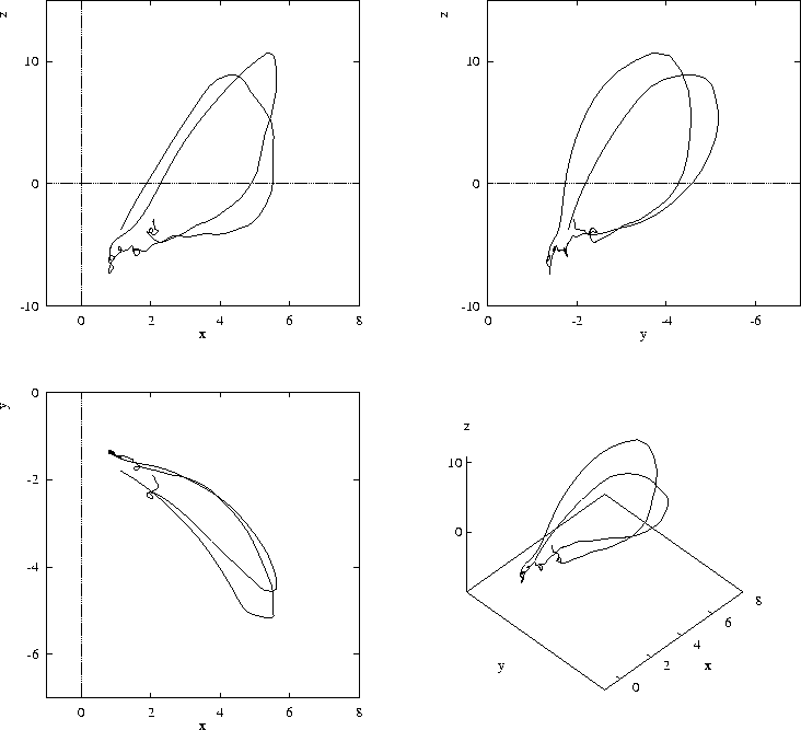
Figure 3:
A piece of trajectory of the quotient system (2) as
extracted from the numerical experiment. Here the Cartesian
coordinates x, y and z stand for ![]() ,
, ![]() and
and ![]() of
(2), respectively.
of
(2), respectively.
Fig. 3 shows a typical projection of the trajectory in the
quotient system in the axes ![]() . One loop typically
consists of a large piece of a fast motion, corresponding to the quick
jumps of the tip trajectory, and a smaller piece closer to the origin
with a slower and oscillatory motion, corresponding to the sharp turns
when the tip nearly stops. This shape of the trajectories in the
quotient system is reminiscent of Shil'nikov chaos near a loop
of a saddle-focus.
Notice that this is close to the mechanism of transition to chaos
via heteroclinic tangle hypothesised in [3, 5] based on the
Barkley's model system.
. One loop typically
consists of a large piece of a fast motion, corresponding to the quick
jumps of the tip trajectory, and a smaller piece closer to the origin
with a slower and oscillatory motion, corresponding to the sharp turns
when the tip nearly stops. This shape of the trajectories in the
quotient system is reminiscent of Shil'nikov chaos near a loop
of a saddle-focus.
Notice that this is close to the mechanism of transition to chaos
via heteroclinic tangle hypothesised in [3, 5] based on the
Barkley's model system.
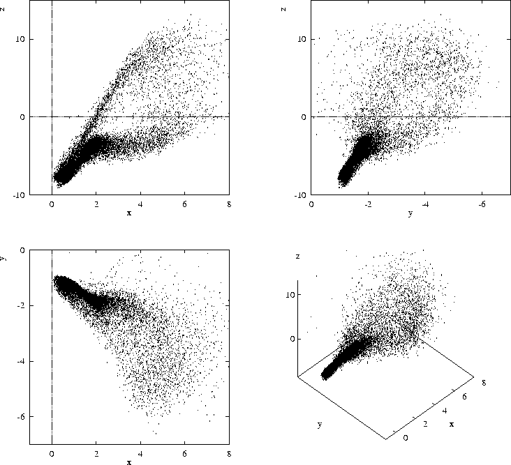
Figure 4:
Attractor of the system (2), i.e. a very long
trajectory from the numerical experiment, shown by dots; coordinates are
the same as in Fig. 3.
Fig. 4 shows the general look of the attractor in the quotient system, in the same coordinates. It is represented by about 12000 points chosen equispaced with interval 10 t.s. or 0.08 t.u.
The accuracy of the computations is enough to see that it is a rather compact set, -- however, its fine structure is smeared out by the numerical noise.
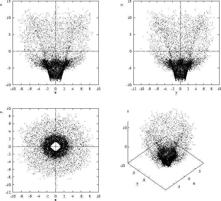
Figure 5:
Attractor in the semi-reduced system extracted
from numerical experiment, with x, y denoting tip velocity
components ![]() and
and ![]() , and z still being
, and z still being ![]() .
.
Fig. 5 shows the attractor in the `semi-reduced' system,
-- same set of points in different coordinates ![]() . It
looks clearly even in both x and y directions. Visually, its
symmetry group may be
. It
looks clearly even in both x and y directions. Visually, its
symmetry group may be ![]() or
or ![]() ; the latter is more likely as
the
; the latter is more likely as
the ![]() -shape of the central hole of the top view should probably be
attributed to influence of the square grid, which is naturally more
noticeable at low propagation speeds.
-shape of the central hole of the top view should probably be
attributed to influence of the square grid, which is naturally more
noticeable at low propagation speeds.
At any rate, the parity of the attractor in the semi-reduced system means that the large-time behaviour should be of Brownian type without directed component. To check this, we measured directly the mean squared walking distance as function of time (Fig. 6).
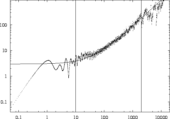
Figure 6:
Mean square of the displacement of the tip I(t) vs time t (dots),
and fitting curve (solid line) in logarithmic coordinates. Vertical
lines show the fitting range.
We assumed ergodicity and calculated the mean squared walking distance by splitting the trajectory from the longest experiment onto pieces of equal length and averaging the square of distance between ends of each piece. The resulting dependence is shown by dots in Fig. 6 (about 3000 points).
Leftmost part of the graph, for t<0.5 t.u., with slope 2 represents differentiability of the trajectories. The range 0.5-10 t.u. is characteristic time range of the attractor in the quotient system. At the times larger than 10 t.u., growth of the displacement due to diffusive motion is seen up to times 2000 t.u. when averaging time intervals become comparable to the length of the experiment, and ergodicity fails.
The long-time walking distance is significantly larger than the typical size of one meandering petal, and so approximations (20) may be sensible in the scale between 10 and 2000 t.u. We fitted the data to (20) and to a more generic dependence
in logarithmic coordinates, using Marquard's method [18] with
equal weights of all points (about 5000) in the range 10-2000 t.u.,
i.e. more than two decades. Fitting by (20) yielded coefficients
![]() and
and ![]() , and good agreement with the
experimental data in two decades of t (see Fig. 6). The
reliability of this approximation can be seen from fitting the same
data to (25), which yielded
, and good agreement with the
experimental data in two decades of t (see Fig. 6). The
reliability of this approximation can be seen from fitting the same
data to (25), which yielded ![]() . Thus,
the experimental dependence of I(t) in a proper range of t is
reasonably approximated by (20), with the hypermeandering
diffusion coefficient
. Thus,
the experimental dependence of I(t) in a proper range of t is
reasonably approximated by (20), with the hypermeandering
diffusion coefficient ![]() , i.e. 40 times less than the
diffusion coefficient of the propagator variable. So, the hypermeander
diffusion is rather intensive and hardly can be attributed to the
numerical noise.
, i.e. 40 times less than the
diffusion coefficient of the propagator variable. So, the hypermeander
diffusion is rather intensive and hardly can be attributed to the
numerical noise.