Example 3: Normal (Gaussian) distribution

A random variable is normally distributed $X\sim N(\mu,\sigma^2)$ when

$$f(x) = \frac{1}{\sqrt{2\pi\sigma^2}}{\rm e}^{-\frac{(x-\mu)^2}{2\sigma^2}}$$ (4.7)

where $x$ is any real number and $\sigma>0$. This is the famous symmetric ``bell-shaped'' curve that provides a remarkably good description of many observed variables. Although often referred to the Gaussian distribution in recognition of the work by K.F. Gauss in 1809, it was actually discovered earlier by De Moivre in 1714 to be a good approximation to the binomial distribution: $X\sim Bin(n,\pi)\approx N(n\pi,n\pi(1-\pi))$ for large $n$. Rather than refer to it as the ``Gaussian'' (or ``Demoivrian'' !) distribution, it is better to simply refer to it as the ``normal'' distribution.

The reason why the normal distribution is so effective at explaining many measured variables is explained by the Central Limit Theorem, which roughly states that the distribution of the mean of many independent variables generally tends to the normal distribution in the limit as the number of variables increases. In other words, the normal distribution is the unique invariant fixed point distribution for means. Measurement errors are often the sum of many uncontrollable random effects, and so can be well-described by the normal distribution.

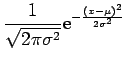
The standard normal distribution with zero mean and unit variance $X\sim N(0,1)$ is widely used in statistics. The area under the standard normal curve, $F(x)$, is sometimes referred to as the error function and given its own special symbol $\Phi(x)$, which can be evaluated numerically on a computer to find probabilities. For example, the probability of a normally distributed variable $X$ with mean $\mu=10$ and $\sigma=2$ being less than or equal to $x=14$ is given by $\Pr(X\leq x)$, which is equal to $\Phi((x-\mu)/\sigma)=\Phi((14-10)/2)=\Phi(2)=0.977$.