Theoretical continuous distributions

Because the estimates are based on a finite number of sample values, the empirical (cumulative) distribution function (e.d.f.) goes up in small discrete steps rather than being a truly smooth function defined for all values. To obtain a continuous differentiable estimate of the c.d.f., the probability distribution can be smoothed using either moving average filters or smoothing splines or kernels. This is known as a non parametric approach since it does not depend on estimating any set of parameters.

An alternative approach is to approximate the empirical distribution function by using an appropriate class of smooth analytic function. For a particular class of function (probability model), the location, spread, and/or shape of the probability density function 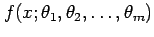$f(x; \theta_1, \theta_2, \ldots, \theta_m)$ is controlled by the values of a small number of population parameters $\theta_1, \theta_2, \ldots, \theta_m$. This is known as a parametric approach since it depends on estimating a set of parameters.

The following sections will describe briefly some (but not all) of the most commonly used theoretical probability distributions.

Figure: Examples of continuous probability density functions: (a) Uniform with $a=-2$ and $b=2$, (b) Normal with $\mu=0$ and $\sigma=1$, and (c) Gamma with $\alpha=2$ and $\beta=1$.